What the solver does
Electromagnetic design studies need thousands of field evaluations, and a single high-fidelity FEM run takes hours. This solver computes magnetic flux density across a 3D grid for arbitrary solenoid geometries in seconds, without generating a mesh. Geometry arrives as STEP files, is fitted to NURBS through OpenCASCADE, and stays in that continuous representation throughout — the Biot–Savart integral uses analytic NURBS tangents rather than finite differences. The output is a parametric dataset at two fidelity levels, built to support multifidelity operator learning.
The method generalises past electromagnetics. Learning a solution operator for a PDE-governed field from a parametric simulation dataset applies to any expensive field simulation; the electromagnetic problem is the controlled testbed, not the point.
One numerical decision worth stating
The ferromagnetic core contributes through surface bound currents, which produces a self-consistency equation solved as a dense 3000×3000 linear system. Iterative solvers were the obvious first choice and the wrong one: GMRES and Richardson both diverge above roughly μᵣ = 5, because the spectral radius of the influence operator exceeds one and the fixed-point iteration stops being a contraction. That is a property of the operator, not of the implementation, so no preconditioner tuning at this size rescues it. Direct LU reaches a residual of 1e-15, and the factorisation is cheap next to the field evaluation. The reason it is documented in the repository is that the failure is silent — an iterative solver still returns a vector.
A loss curve that looked fine
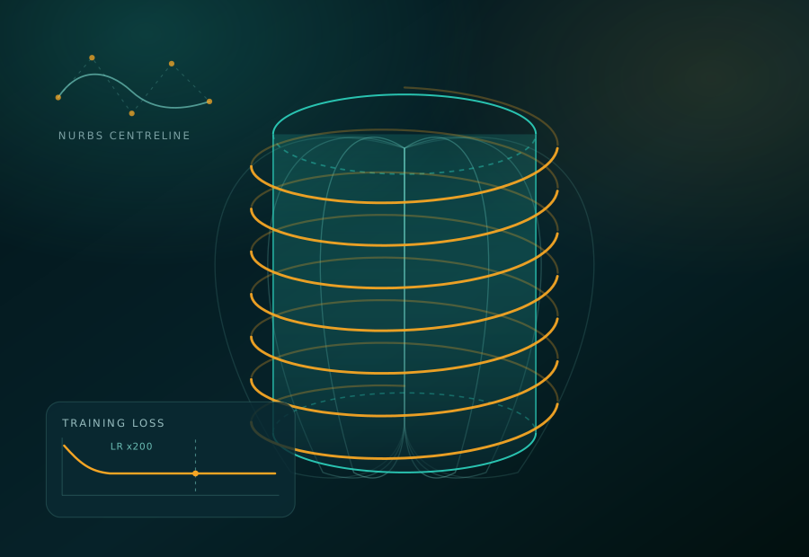
The surrogate is a graph-network DeepONet with a SIREN trunk and a physics residual, trained on two T4s. Training and validation loss were bit-identical to five significant figures for twenty-five consecutive epochs — including across a scheduler warm restart that raised the learning rate by a factor of two hundred. A network that is learning cannot reproduce an identical five-figure epoch mean under reshuffled minibatches and a 200× learning-rate change. Nothing in the logs said so; the numbers were finite, small and stable, which is what a converged run looks like.
The guard that hid the failure
The immediate cause was scale. Core conductivity of order 10⁷ S/m and coil radius of order 10⁻² m were fed into the same linear layer — nine orders of dynamic range — pushing activations to the floating-point ceiling. Gradient clipping then converted a single infinite gradient into model-wide NaN, because the clip coefficient becomes zero and infinity times zero is not a number.
What made it invisible was the safeguard. Every layer ended in a call that rewrites non-finite values to finite ones. Its derivative in PyTorch is the incoming gradient multiplied by a finiteness mask, so a blow-up is never surfaced as a NaN loss — it is quietly replaced by a constant carrying zero gradient. The network emitted the same output for every input, the loss reduced to a function of the data alone, and it stayed there. The measures taken to make training robust are precisely what prevented anyone from noticing it had stopped.
Confirming it from the checkpoint
Rather than infer the mechanism, the saved checkpoint was parsed at the tensor-storage level. The optimizer held state for only forty-five of sixty-one parameter tensors. Because AdamW allocates state lazily on a parameter's first gradient, the sixteen without state had never received one. They mapped exactly onto a graph structure the code constructed and then never used — an entire message-passing sub-network wired to nothing, invisible in the loss and invisible in the parameter count.
The physics term was measuring the wrong quantity
Separately, the physics residual contradicted the solver it was meant to agree with. It computed magnetisation from the material field alone with a permeability factor in the wrong place, where the solver's own constitutive law uses the total field — understating the bound surface current by a factor of the relative permeability, three orders of magnitude for the cores in this dataset.
The replacement was checked against a closed-form solution rather than accepted on inspection. A uniformly magnetised cylinder has bound currents identical to a solenoid, whose on-axis field is known exactly, so a single test exercises the constitutive law, the cross-product sign, the quadrature weights and the integral kernel together. The corrected scheme converges at second order to a relative error of 3.9e-5 where the original sat at 8.0e-2. That test now runs in continuous integration on every push, needs no FEM licence, and finishes in seconds.
What it does not settle
The corrected training pipeline is implemented but has not been retrained, so no surrogate accuracy figure is claimed and none appears in the repository. The verification suite establishes that the solver computes the formulation it says it computes; it does not establish accuracy against a full-Maxwell reference outside the analytic test family, and the ANSYS/COMSOL cross-check remains open. The low and high fidelity labels still describe grid resolution and solve cost rather than measured error, and are marked as such.
Why this matters beyond electromagnetics
A model that has stopped learning and a model that has converged produce the same artefact: a flat loss curve made of small finite numbers. Telling them apart took a warm restart the network should have responded to, an epoch mean identical to more digits than noise allows, and a checkpoint read at the byte level. The transferable habit is treating defensive code as a hypothesis rather than a guarantee — the exception handlers, NaN guards and clipping rules written to keep a pipeline alive are also the ones that let it die quietly. It is the same lesson as the rocket-motor study approached from the other side: there, a solver went silent and wrote nothing; here, a trainer went silent and wrote plausible numbers. The second is harder to catch.